so-you-think-you-can-code-2025

💡 AI Transparency Disclosure: I used an AI assistant to polish up the text and code comments in this post. The code itself, and the initial, unrevised content of the blog post, were entirely written by me.

Introduction to Path Tracers

Intended audience: Shader developers who have written a few ray marchers and are curious about path tracing.

Note: This article shows selected code snippets to explain important concepts. Complete source code is available via the Shadertoy and source file links.

Path Tracers vs Ray Marchers

If you’ve been exploring shaders on shadertoy.com, you’ll notice that most use ray marching (or sphere marching). Ray marchers allow for complex geometries, even fractals, but achieving nice, interesting shading typically requires various tricks. Getting good-looking shadows and diffuse lighting takes effort, while color bleeding and multiple light sources demand additional hacks and tinkering, like trying to manually calculate how your Christmas lights should illuminate each ornament.

Path tracers handle these effects more naturally because they more closely emulate how light actually behaves in nature. Imagine tracking how light from a string of Christmas bulbs bounces around a room, illuminating everything with colored reflections. While real photons travel from light sources to our eyes, path tracers work backwards, tracing from the eye until hitting a light. This reversed but physically accurate approach means effects like soft shadows, color bleeding, and global illumination emerge automatically from the algorithm itself.

The trade-off is that path tracers work best with explicit geometry like spheres, planes, and triangles, rather than the infinite fractal complexity that ray marchers excel at. You need simpler scenes to maintain real-time performance.

Here’s how it works: we send a ray from the eye into the scene and let it bounce, choosing each new direction randomly (using a distribution called uniform Lambertian) until it either hits a light source or escapes the scene. Because of this randomness, we need to send many rays per pixel and average the results to reduce noise.

Let’s Start Coding a Simple Ray Tracer

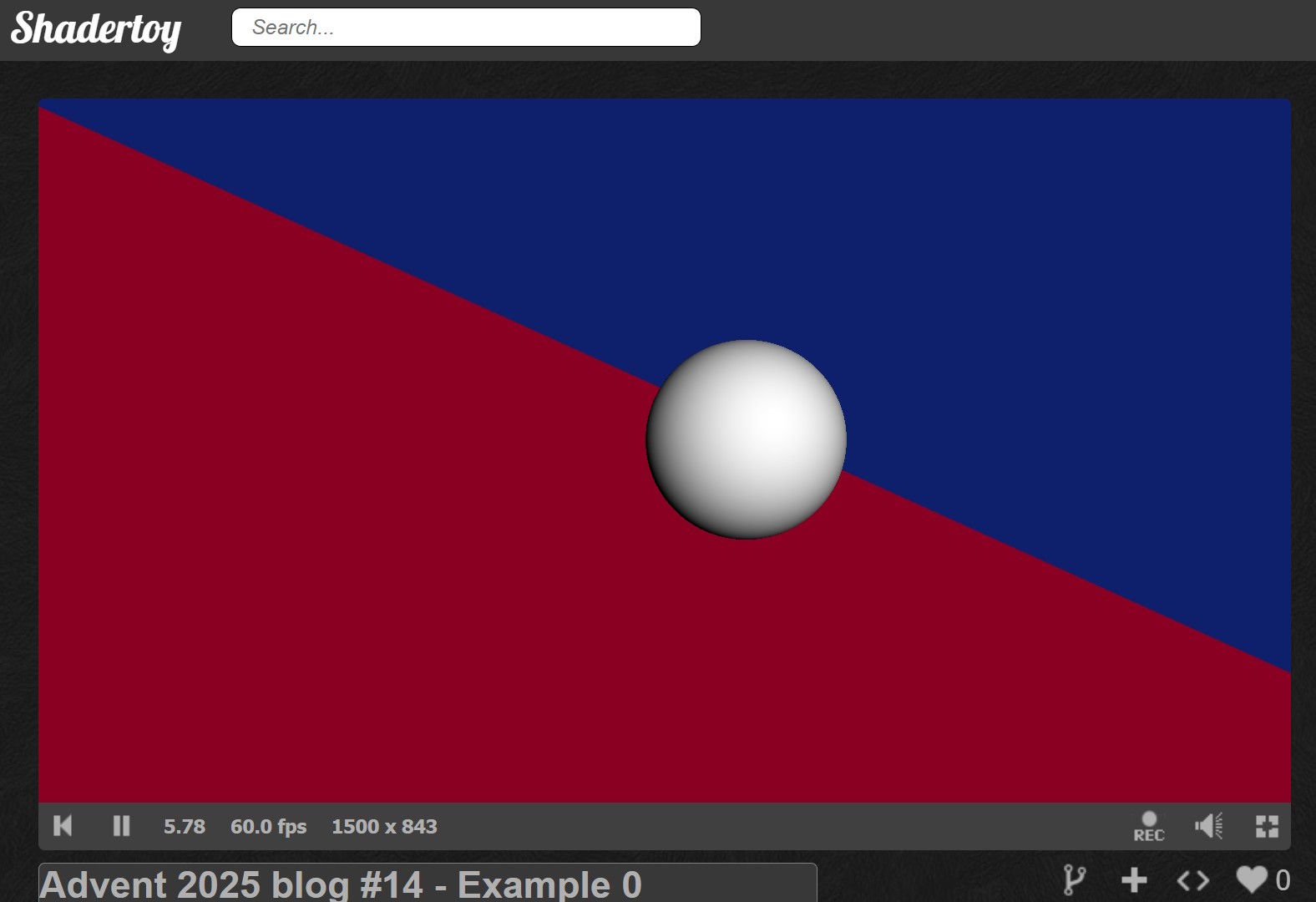
Let’s build a simple ray tracer that traces two planes and a sphere using basic shading so we can see the objects. This simple ray tracer will serve as our foundation. In later parts, we’ll replace this direct lighting with path tracing.

We’ll work with normalized screen coordinates p (ranging from -1 to 1) to determine which direction each pixel should look. First, we need to set up our ray based on the camera origin and where it’s looking:

const vec3
  // Camera origin (eye position)
  ro        = vec3(4,4,-6.)
  // Look-at point (camera target)
, la        = vec3(0,.5,-2.)
  // Camera forward vector (viewing direction)
, cam_fwd   = normalize(la - ro)
  // Camera right vector (horizontal axis)
, cam_right = normalize(cross(cam_fwd, vec3(0,1,0)))
  // Camera up vector (vertical axis)
, cam_up    = cross(cam_right, cam_fwd)
;
vec3
  // Ray direction through pixel (camera-to-world transform)
  rd            = normalize(-p.x*cam_right + p.y*cam_up + 2.*cam_fwd)
;

For a plane at a fixed coordinate, we solve for where the ray crosses it:

  float
    // Distance to floor intersection (y = -1 plane)
    t_floor   = (-1. - ro.y) / rd.y
    // Distance to wall intersection (z = 1 plane)
  , t_wall    = (1. - ro.z) / rd.z
  , t_sphere  = ray_unitsphere(ro - sphere_center, rd)
  ;

Finding ray-sphere intersection is more involved, so I borrowed some code from IQ:

// License: MIT, author: Inigo Quilez, found: https://iquilezles.org/articles/intersectors/
float ray_unitsphere(vec3 ro, vec3 rd) {
  float
    b=dot(ro, rd)
  , c=dot(ro, ro)-1.
  , h=b*b-c
  ;
  if(h<.0) return -1.;
  return -b-sqrt(h);
}

Now we have three intersection distances. We initialize t to a large value (representing infinity), then check each primitive. Any positive intersection distance smaller than our current t becomes our new closest hit:

// Find closest intersection by testing all primitives directly
// We keep the smallest positive t value - this is the nearest surface hit
if(t_floor>0.   && t_floor<t)   { t=t_floor;  normal=vec3(0,1,0); }
if(t_wall>0.    && t_wall<t)    { t=t_wall;   normal=vec3(0,0,-1); }
if(t_sphere>0.  && t_sphere<t)  { t=t_sphere; normal=normalize(ro+rd*t_sphere-sphere_center);}

For basic shading, we use Lambertian diffuse lighting, which makes surfaces brighter when facing the light. We place a light source above and to the side of the scene, then assign colors based on what we hit:

// Lambertian diffuse shading (cosine falloff)
diffuse = max(0., dot(normal, light_dir));
if(t==t_floor) {
  // Give floor a reddish color
  color = vec3(1,0,.25);
} else if(t==t_wall) {
  // Give wall a bluish color
  color = vec3(0,.25,1);
} else if(t==t_sphere) {
  // The sphere is white
  color = vec3(1);
} else {
  // Missed the scene
  color=vec3(0);
}
color*=diffuse;

Here’s the complete shader running in ShaderToy:

ShaderToy link Source code link

The scene works, but it looks flat and lifeless. Why? Surfaces don’t block light from each other, so there are no shadows. There’s no sense of how nearby geometry darkens corners. What’s missing are shadows and ambient occlusion.

We could fake these effects with various tricks to make it look decent, but since this series is about path tracing, let’s see how these effects emerge naturally from the algorithm. In the next section, we’ll add random bounces to our rays and implement a simple path tracer.

📢 Expect Noise

Path tracing uses randomness (the Monte Carlo method). The trade-off for physically accurate lighting is the resulting image noise.

We can reduce this noise by increasing the number of samples (at the cost of framerate) or by applying a filter. In this example, we use a simple temporal accumulation. This technique blends new frames with old ones to average out the speckles over time.

A Simple Path Tracer

Unlike our basic ray tracer that cast one ray and did direct lighting, the path tracer traces complete light paths with multiple bounces. This is what gives us those natural shadows and lighting effects.

To simulate diffuse lighting with soft shadows and color bleeding, we’re going to cast multiple rays and randomly bounce them off surfaces until they hit a light source or miss the scene.

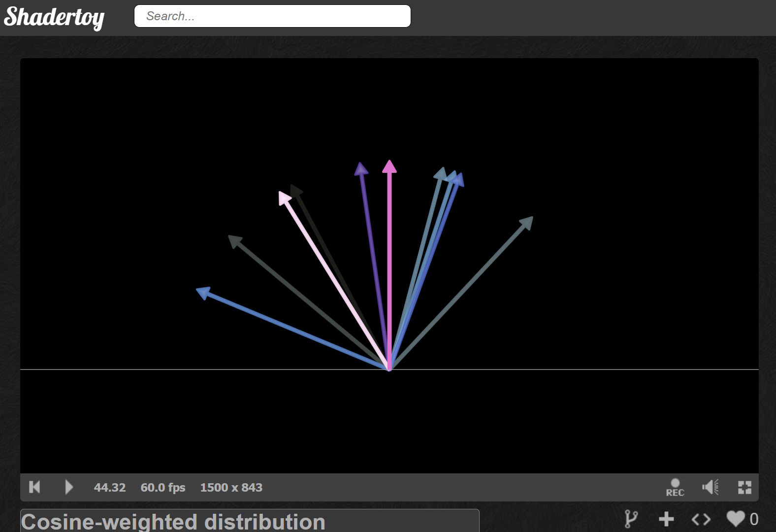
But how do we choose the random directions? We’ll use a cosine-weighted distribution (often called a Lambertian distribution in this context). Think of it like this: when light hits a rough surface, it scatters in all directions, but more photons bounce close to perpendicular (the normal) than grazing along the surface (the tangent).

ShaderToy link

I borrowed some code from a very cool path tracer shader by 0b5vr.

The uniform_lambert function generates directions using two random numbers. The first picks an angle spinning around the hemisphere (0 to 2π). The second determines how far from the normal the ray goes. By taking its square root, we get more rays near the normal, which is exactly what diffuse surfaces do.

float g_seed;

// License: Unknown, author: 0b5vr, found: https://www.shadertoy.com/view/ss3SD8
float random() {
  float i = ++g_seed;
  return fract(sin((i)*114.514)*1919.810);
}

// License: Unknown, author: 0b5vr, found: https://www.shadertoy.com/view/ss3SD8
// Generates a cosine-weighted random direction in the hemisphere above normal n
// The sqrt() on cost creates the cosine weighting - more samples near the normal
vec3 uniform_lambert(vec3 n){
  float
    // Random azimuthal angle: spin around the hemisphere (0 to 2π)
    p=PI*2.*random()
  , // Polar angle cosine: sqrt gives cosine-weighted distribution for diffuse
    cost=sqrt(random())
  , // Polar angle sine: derived from cos via trig identity
    sint=sqrt(1.-cost*cost)
  ;
  // Convert from spherical (local) to Cartesian, then transform to world space
  // Local space: Z=up from surface, X/Y=tangent plane
  return orth_base(n)*vec3(cos(p)*sint,sin(p)*sint,cost);
}

What is orth_base? It’s a function that builds a coordinate system where the z-axis points along the surface normal. This lets us work in ‘surface space’ where generating hemisphere samples is simple.

// License: Unknown, author: 0b5vr, found: https://www.shadertoy.com/view/ss3SD8
// Returns a rotation matrix that transforms from local space (where Z=up) to world space
mat3 orth_base(vec3 n){
  // Assumes n is normalized
  vec3
    // Pick a helper vector that won't be parallel to n
    // Avoids gimbal lock when normal points straight up/down
    up=abs(n.y)>.999?vec3(0,0,1):vec3(0,1,0)
  , // First tangent: perpendicular to both 'up' and normal
    x=normalize(cross(up,n))
  , // Second tangent: perpendicular to both normal and first tangent
    // Completes the right-handed coordinate system
    y=cross(n,x)
  ;
  return mat3(x,y,n);
}

These are the most complex functions in the shader, but the good news is they’re the same for every path tracer you’ll write in your career.

The path tracer traces one complete light path per loop iteration. Each path starts at the camera, bounces around until hitting a light (or escaping), and contributes its radiance to the final pixel color. The main loop looks like this:

// Initialize path from camera
prev_pos    = ro;
prev_normal = rd;
throughput  = 1.;

// Path tracing loop: trace one path per iteration
for(int i=0; i<150; ++i) {
  // Ray-plane intersection: floor at y = -1
  t_floor   = (-1. - prev_pos.y) / prev_normal.y;
  // Ray-plane intersection: wall at z = 1
  t_wall    = (1. - prev_pos.z) / prev_normal.z;
  // Ray-sphere intersection: unit sphere at sphere_center
  t_sphere  = ray_unitsphere(prev_pos - sphere_center, prev_normal);

We check when to terminate the ray. Termination happens if we missed the scene, the throughput has dimmed below 0.1 (meaning further bounces won’t contribute visibly), or we hit the glowing stripe on the wall.

When we terminate, we check if we hit the emissive wall stripe. If so, we add its contribution to the color, accounting for the current throughput. Then we reset the ray position and direction to the camera origin, reset the throughput, and increment the sample counter.

// Check path termination conditions
missed      = t==1e3 || throughput<1e-1;
// Wall stripe emissive
hit_stripe  = t==t_wall && abs(pos.x)<1.;

// Early exit: first ray missed entire scene
if(i==0 && missed) {
  break;
}

// Path completed: we hit a light source or missed
if(missed || hit_stripe) {
  if(hit_stripe) {
    // White emissive stripe
    radiance += throughput*vec3(1);
  }

  // Start new path from camera
  prev_pos    = ro;
  prev_normal = rd;
  throughput  = 1.;
  ++samples;
  continue;
}

If we shouldn’t terminate, we bounce the ray off the surface. We choose the new direction randomly using the uniform Lambertian distribution to emulate diffuse light. We set the ray direction to this randomized direction, multiply the throughput by 0.4 (meaning the surface absorbs 60% of the light and reflects 40%, this is how surfaces get their brightness), and advance the position slightly along the normal to prevent self-intersection.

// We hit a non-emissive surface: compute next path segment

// Cosine-weighted hemisphere sample for diffuse
diffuse_dir = uniform_lambert(normal);

// Diffuse bounce
prev_normal = diffuse_dir;
throughput *= .4;

// Advance path with small offset to prevent self-intersection
prev_pos = pos + 1e-3*normal;

Finally, we divide by the number of samples to get the average radiance, clamp negative values, and blend the current frame with the previous frame (temporal accumulation) to smooth out the noise. Each new frame adds more samples, gradually refining the image, like how a photograph gets clearer with longer exposure. We apply gamma correction (square root as a rough approximation) to convert from linear light values to sRGB, which is what monitors expect.

// Monte Carlo estimator: average over all samples
radiance /= max(samples, 1.);
// Clamp to prevent NaN propagation in temporal accumulation
radiance = max(radiance, 0.);
// Temporal accumulation: exponential moving average for variance reduction
radiance = mix(radiance, prev_frame*prev_frame, .5);
// Gamma correction (linear to sRGB approximation)
radiance = sqrt(radiance);

return vec4(radiance, 1.);

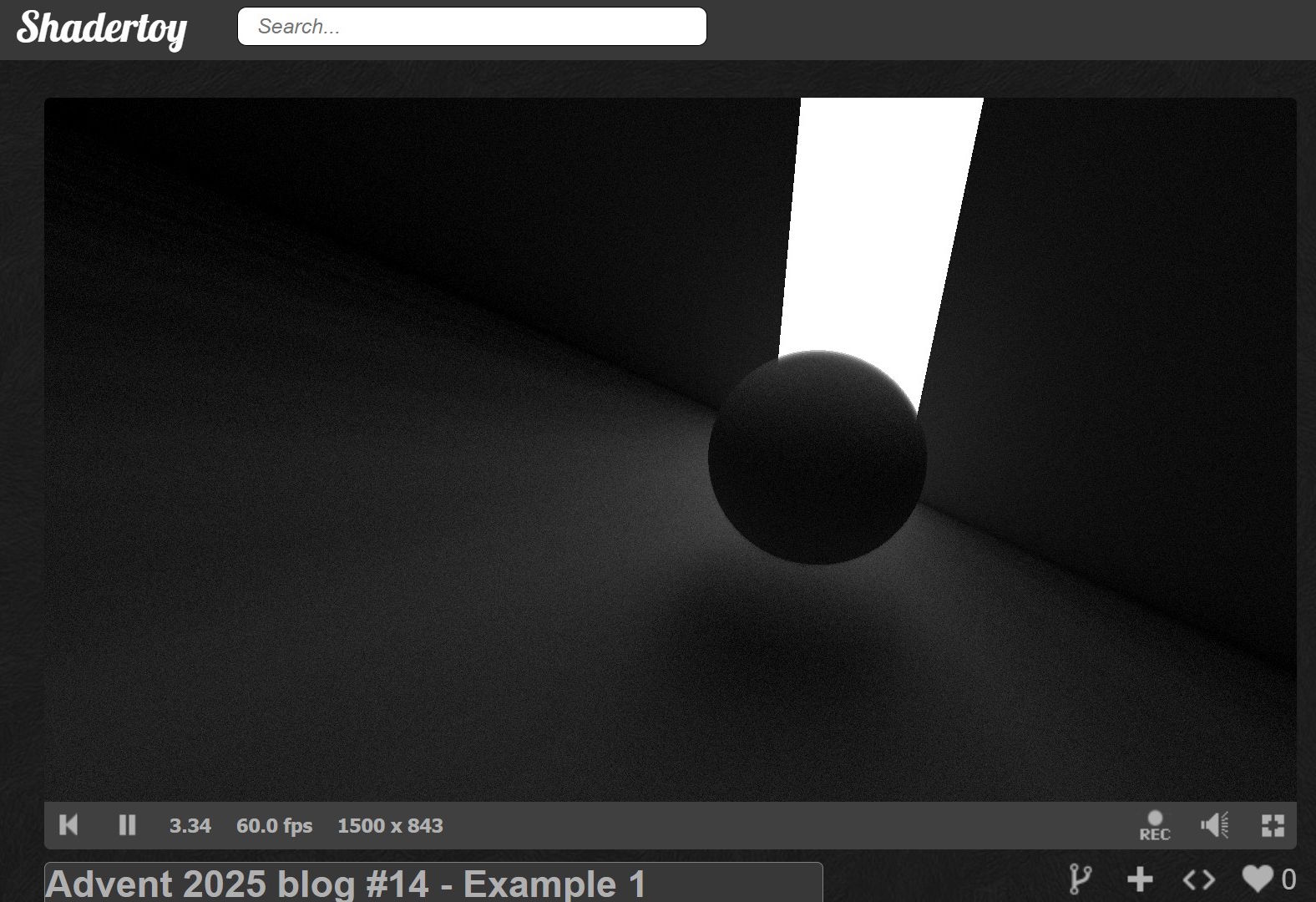
Here’s the complete shader running in ShaderToy. Note that it’s a multipass shader so we can sample the previous frame for temporal accumulation. You’ll find most of the code under the Buffer A tab.

ShaderToy link (see Buffer A for the core implementation) Source code link

Notice how we get soft shadows, light falloff with distance, and color bleeding without explicitly coding for any of these effects as we would have needed to in a ray marcher. The physics of light bouncing handles it all automatically. That’s the magic of path tracing!

In the final step, we’re going to add colored surfaces and reflections to the scene. We’ll also get anti-aliasing for free.

Decking the Halls

As mentioned, let’s add anti-aliasing by introducing noise when computing the ray direction. We do this by randomly offsetting where within each pixel we sample. Instead of always shooting through the pixel center, we jitter the position slightly. Since we’re accumulating multiple samples, edges naturally blend together.

vec3 noisy_ray_dir(vec2 uv, vec3 cam_right, vec3 cam_up, vec3 cam_fwd) {
  // Jitter sample position within pixel for antialiasing (stochastic sampling)
  uv += (-1. + 2.*vec2(random(), random())) / RENDERSIZE.y;
  return normalize(-uv.x*cam_right + uv.y*cam_up + 2.*cam_fwd);
}

Next, we’ll add more light sources by dividing the wall into a grid. We hash each cell’s coordinates to give it random properties. Cells with a hash above 0.9 become colorful lights, creating a festive grid of glowing squares on the wall.

We’ll also add a yellow stripe on the floor. This gives us warm, colored light bouncing up onto the wall and sphere.

// Transform wall intersection to scrolling texture space
wall_pos  = pos.xy - vec2(TIME, 0.5);
// Compute cell indices for procedural tiling
cell_idx  = floor(wall_pos + .5);
// Compute position within cell
cell_uv   = wall_pos - cell_idx;
// Hash cell indices for material properties
cell_hash = hash(123.4*cell_idx);

// Check path termination conditions
missed      = t==1e3 || throughput<1e-1;
// Wall cells with hash > 0.9 are emissive
hit_light   = cell_hash>0.9 && t==t_wall;
// Floor stripe at z = -2 is emissive
hit_stripe  = t==t_floor && abs(pos.z+2.)<.1 && sin(wall_pos.x)>0.;

// Early exit: first ray missed entire scene
if(i==0 && missed) {
  break;
}

// Path completed: we hit a light source or missed
if(missed || hit_light || hit_stripe) {
  if(hit_light) {
    // Procedural light color based on cell hash and distance
    radiance += throughput*(1.1 - length(cell_uv) + sin(vec3(2,1,0) + TAU*fract(8667.*cell_hash)));
  }
  if(hit_stripe) {
    // Yellow emissive stripe
    radiance += throughput*vec3(1,.5,0.);
  }

  // Start new path from camera
  prev_pos    = ro;
  prev_normal = noisy_ray_dir(p, cam_right, cam_up, cam_fwd);
  throughput  = 1.;
  ++samples;
  continue;
}

Finally, we’ll make surfaces reflective. In reality, all surfaces become mirror-like at grazing angles. This is called the Fresnel effect. You can see this if you stand next to a lake: looking straight down, you see through the water to the bottom. But looking toward the horizon, the water becomes a perfect mirror.

We compute a Fresnel factor that increases as the viewing angle gets shallower. We use this factor to randomly choose between reflection and diffuse scattering. Rather than tracing both paths (which would require recursion that GLSL doesn’t support), we randomly pick one and weight the result appropriately. Over many samples, this averages out to the correct result.

Some surfaces are always reflective regardless of angle: the sphere acts as a chrome ball, and about half the wall cells become perfect mirrors (determined by their hash). This creates interesting reflections throughout the scene.

Perfect reflections retain 90% of the light’s energy (shiny surfaces absorb very little), while diffuse reflections retain only 40% (rough surfaces absorb more).

// We hit a non-emissive surface: compute next path segment

// Schlick's approximation for Fresnel reflectance
fresnel = 1. + dot(prev_normal, normal);
fresnel *= fresnel;
fresnel *= fresnel;
fresnel *= fresnel;

// Ideal specular reflection direction
reflect_dir = reflect(prev_normal, normal);
// Cosine-weighted hemisphere sample for diffuse
diffuse_dir = uniform_lambert(normal);

if(
    // Russian Roulette path splitting approximation:
    // randomly choose specular or diffuse based on Fresnel term
    random() < fresnel
    // Some wall cells are mirrors
  ||(fract(cell_hash*7677.)>0.5 && t==t_wall)
    // Sphere is reflective
  || t==t_sphere
  ) {
  // Specular bounce
  prev_normal = reflect_dir;
  throughput *= .9;
} else {
  // Diffuse bounce
  prev_normal = diffuse_dir;
  throughput *= .4;
}

// Advance path with small offset to prevent self-intersection
prev_pos = pos + 1e-3*normal;

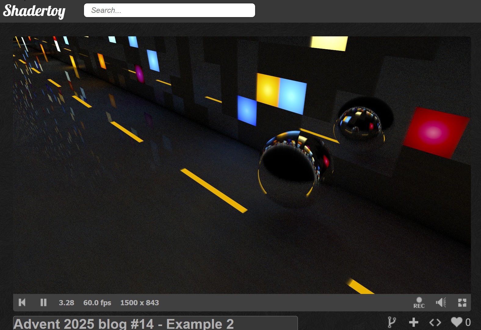
With all these pieces together, we get a scene with anti-aliased edges, colorful lights scattered across the wall, warm yellow illumination from the floor, and a shiny sphere reflecting everything around it.

Here’s the complete shader running in ShaderToy. Note that it’s a multipass shader so we can sample the previous frame for temporal accumulation. You’ll find most of the code under the Buffer A tab.

ShaderToy link (see Buffer A for the core implementation) Source code link

Finally, some festive colors! The scene now features a shiny chrome sphere bouncing along the floor like a fallen Christmas ornament. We added just a few key features, anti-aliasing, multiple colored lights, and reflective surfaces, but the visual transformation is dramatic.

Remember our basic ray tracer with its flat, shadowless surfaces? Compare that to this scene where light dances between surfaces, colors bleed naturally, and reflections appear automatically. Look at what emerged naturally: crisp anti-aliased edges, colorful light bleeding from the wall squares onto the floor, and subtle reflected illumination when the sphere passes over the yellow stripe.

All these effects, the soft shadows, the color mixing, the reflections, emerged from the same simple algorithm: bounce rays randomly until they hit light.

Your Turn

Thanks for following this guide! Now it’s your turn to experiment…

Try modifying the shader: change the surface colors, add more geometry, adjust the Fresnel factor, or make different surfaces reflective. Break things, fix them, and watch how light behaves. The best way to truly understand path tracing is to play with it yourself.

Happy holidays, and happy rendering! May your frames be noise-free and your bounces be plentiful. ✨

🫶 mrange 🫶

🎄What’s Under the Christmas Tree?!🎄

Almost forgot the presents! Here are two techniques that might spark some interesting experiments.

Diffuse Reflection Tricks

The physically correct approach passes the surface normal to uniform_lambert:

diffuse_dir = uniform_lambert(normal);

But here’s a fun deviation: try passing the reflected ray instead:

diffuse_dir = uniform_lambert(reflected_ray);

This isn’t physically accurate, but it often produces surprisingly appealing results. You can sharpen the effect further by focusing the distribution. Use cost = pow(random(), 0.1) in your uniform_lambert function instead of sqrt.

Faster Lambert Approximation

Our current implementation follows the standard cosine-weighted distribution. But catnip from the FieldFX discord shared an elegant approximation that’s both easier to remember and faster to compute:

// License: Unknown, author: catnip, found: FieldFX discord
vec3 point_on_sphere(vec2 r) {
  r = vec2(PI*2.*r.x, 2.*r.y-1.);
  return vec3(sqrt(1. - r.y * r.y) * vec2(cos(r.x), sin(r.x)), r.y);
}

// License: Unknown, author: catnip, found: FieldFX discord
vec3 uniform_lambert(vec2 r, vec3 n) {
  // r is 2 random numbers
  return normalize(n*(1.001) + point_on_sphere(r)); // 1.001 avoids NaN in rare cases
}

🎁Both gifts are yours to unwrap and experiment with. See what they do to your renders!